Are you tired from constantly living in the dark, fully unaware of the current Gamma Exposure?
Are you frustrated from having to guess the Zero Gamma level ALL THE TIME?
Are you annoyed from not knowing what the f*ck all of this even means!?!
I know, I was.
Hello, my name is Sergei.
And today, I will show you how YOU can change YOUR life, once and forever!
After this 10-minute tutorial, you will be able to take full control of your gamma needs and live the life YOU want.
Impress your boss, colleagues, friends, spouse, children, dog!
By the end of this post, you will be able to:
- Create a simple spot gamma chart for your favourite stock index.
- Compute its total gamma exposure.
- Construct a sleek-looking gamma profile chart.
- Calculate a Zero Gamma level (aka Flip Gamma).
!!! AND !!!
- UNDERSTAND WHAT ALL OF THIS MEANS!!!11
Now, I know what you're thinking:
"Oh Sergei, it sounds too good to be true! We'll probably need an expensive Bloomberg Terminal for that! And some premium exchange options data... And a powerful quantum computer!"
Right?
NO!
WRONG!
We will calculate gamma exposure using simple tools that you can find around the house!
That's right!
So put that Bloomberg Terminal away and get your power tools out!
It's time to do some maths!

Calculating Spot Gamma Exposure
First of all - if you feel like refreshing your understanding of gamma and how it impacts the market, you can take a look at this non-technical post.
In this article, we'll finally get our hands (and minds) dirty and talk about the calculations behind those charts.
Let's start by constructing a simple spot gamma visualizer tool.
For that, we'll need:
- A cup of coffee ☕️
- Some options data
- Excel
Since coffee and Excel are easy to come by, let's talk about the options data. At the most basic level, we'll need the standard option chain stuff, like strikes, expiries and open interest (OI).
But we'll also need to get our hands on the unit gamma for each option. And gamma is a bit more challenging to find. Sometimes it's provided on the option chain, along with implied volatility (IV) and deltas. But it could be that it's not offered for your specific asset, and you'll need to calculate it manually. If that's the case for you - keep reading, as we'll be calculating gammas later on anyway.
For the rest of the thread, I'll use $SPX index as an example.
Luckily, for US stocks, CBOE provides an excellent options data tool, which includes gamma, among other things. This is available here: https://www.cboe.com/delayed_quotes
Search for "SPX" -> click on Options tab -> set Options Range == All -> set Expiration == All -> click View Chain. To download the entire options chain, scroll all the way down, and click on Download CSV.
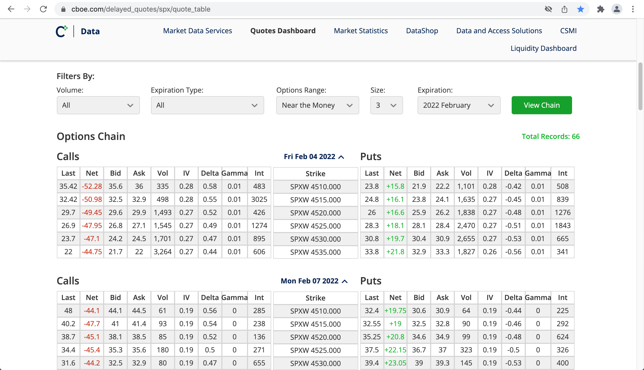
We now have an entire snapshot of the SPX options data in Excel.
Fantastic! Well done!
I think we all deserve a break now. *slurp* ☕️
While we're enjoying the coffee, a couple of words about this data.
First, note that the open interest figures are updated once per day. Almost always, this will be yesterday's data. Nonetheless, I found that CBOE updates it earlier than other sources and frequently shows yesterday's data, while the rest show OI from the day before.
Secondly, this data is best served fresh. It's better to download it during market hours, as overnight data from the last close can be a bit noisy. I had trouble replicating some gamma values obtained after the close.
Alright, break over. Back to Excel.
We want to find out two things:
- How much gamma the dealers are sitting on across the index levels, and
- What's their current total gamma exposure.
For these calculations, ideally, we need to know how many of each particular option the dealers hold. Unfortunately, they're a secretive bunch and keep their cards close to their chest. Hence, we need to make an assumption about that.
A crude approximation is that the dealers are long the calls and short the puts, which is true to some expend on an index level. For single-stocks, it's more debatable, as the street can be short the calls due to some speculative buying frenzy.
*cough* Telsa *cough*
It is possible to build up a more accurate dealer positioning picture from trade reporting data, however, it's not for the faint-hearted.
So, we'll assume that calls carry positive gamma and puts negative.
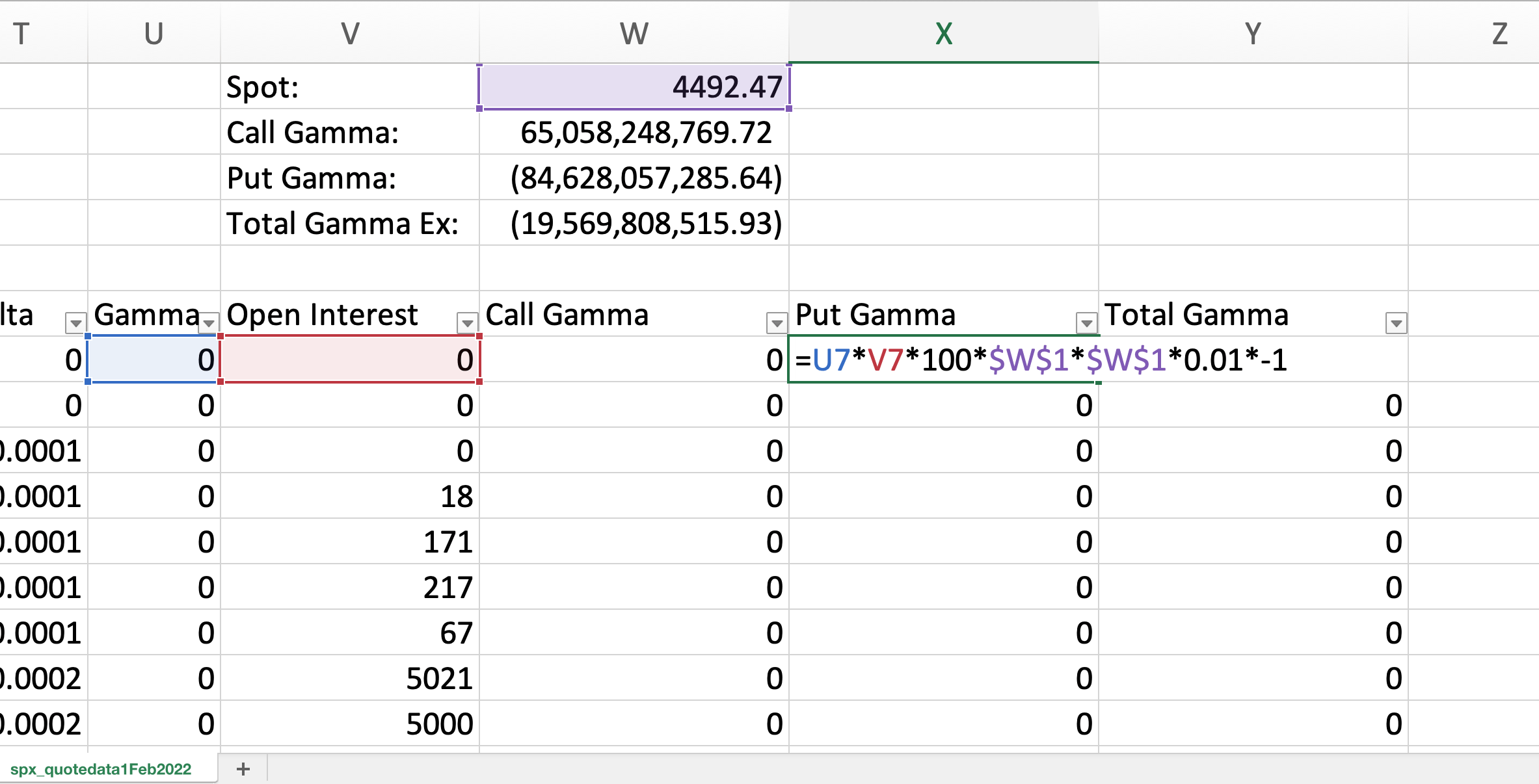
Let's now calculate the total gamma contribution from each option. The formula is:
Option's Gamma * Contract Size * Open Interest * Spot Price * (-1 if puts)
This gives the total option's change in delta per ONE POINT move in the index. To convert into percent, we must multiply by how many points 1% is. Hence, we multiply by 1% * Spot Price, giving the final formula:
Option's Gamma * Contract Size * Open Interest * Spot Price ^ 2 * 0.01
Summing gamma contributions across the options gives us the total gamma exposure. Doing this in Excel for 1 Feb 2022 gives me -$19Bn.
In plain English:
Option dealers need to SELL $19Bn worth of $SPX index for each 1% move DOWN, and BUY $19Bn for each 1% move UP.
Frequently the gamma exposure is an overstatement, and the actual delta-hedging flows are typically smaller than this calculation would imply.
This is because investors:
- Also sell puts for yield (structured products)
- Buy calls for leverage
- Trade spreads and combos
So that's something to keep in mind.
Let's now look at how gamma exposure is distributed across strikes and expiries. Select the area with the headings and the data and click on Insert -> Pivot Table.
Ehmmm.... what are you waiting for? Go on! You can do this one ;)
Pivot Table allows us to easily aggregate the gamma values for a range of strikes and expiries. Under PivotTable Fields, drag-and-drop Strike into the Rows and drag Total Gamma into Values. This will give you a total gamma exposure per strike!
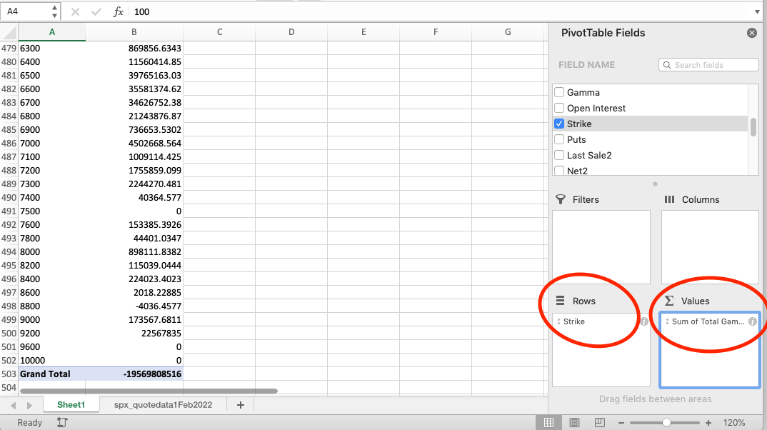
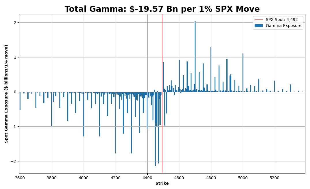
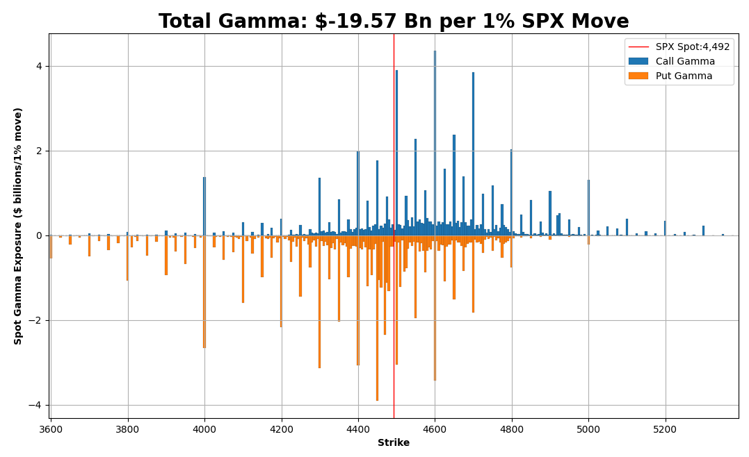
If you now click on the Pivot Table Analyse tab -> Pivot Chart, you'll get an excellent visualisation. The chart below shows how much gamma is outstanding at each strike from the point of view of the current spot. This is why it's called spot gamma exposure. Each bar represents how much delta needs to be bought or sold if the market moves by 1% from where it is now.
And the beauty of the Pivot Table is that you can effortlessly slice and dice the data any way you want. Want to see the largest gamma expiries? No problem -> remove the Strikes from Rows and add Expiration Date instead.
Boom!
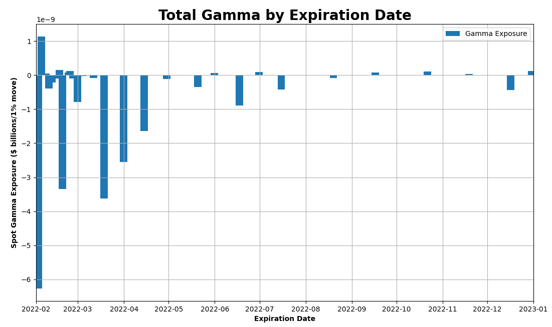
Want to see gamma for calls and puts separately? Replace Total Gamma with Put Gamma and Call Gamma and put the Strike back in place of Expiration Date.
Boom!
I know, I know - MIND BLOWN!
But that's NOT all, folks!
We were only getting warmed up for what lies ahead!
Are you ready?
Calculating Gamma Profile and Zero Gamma Level
So far, we calculated the gamma exposure for the current spot level only. But what if we wanted to know an approximate gamma exposure if the market drops by 10%? Or how about if it rallies by 10%? Would the dealers be short or long gamma, and at what point would it flip?
This is a slightly more complex question since we must compute the gamma exposure not just for the current spot but across the index levels.
As in, we need to do that Excel calculation for different spot values.
Well, that's great news - we already know how to do that!

Yeah... there is just one tiny problem....
When we change the spot, options gammas will change. This means we can no longer use the same gammas so thoughtfully provided by CBOE.
Those have to be recalculated.
For every option.
For every spot price.
And while it's possible to do it in Excel, it's a bit of an overkill... It's time to dig into your toolbox and pull out some Python.
So how do we go about that?
Allow me to demonstrate.
I want you to meet my little friend.
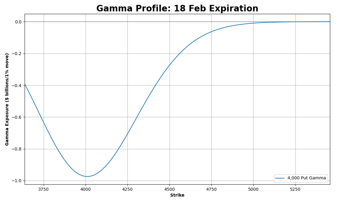
This is a 4,000 put option, expiring on 18 Feb (Sorry, he's a little shy...)
Using a Black-Scholes formula, we can calculate its gamma since we have most of the ingredients we need. The CBOE data provides strikes, expiries and, most importantly, IV levels for each option. We'll use those.
We also need to source the interest rate data (ideally swap rates) and a projected dividend yield. I leave this as an exercise for the reader (Muahahahaha!!!)
In this example, we'll set rates and divs to zero (or to 1.5-2% to be closer to the current levels for $SPX). Although, they don't really impact the final figures that much. A billion here, a billion there, not a big deal... Blame it on the rounding error.
Let's come back to our 4,000 put.
Hi there!
So for this option, we do the following:
- Download its data into Python.
- Apply the Black-Scholes and calculate unit gamma for a range of spot levels.
- Using unit gamma, calculate the total gamma exposure at each spot price.
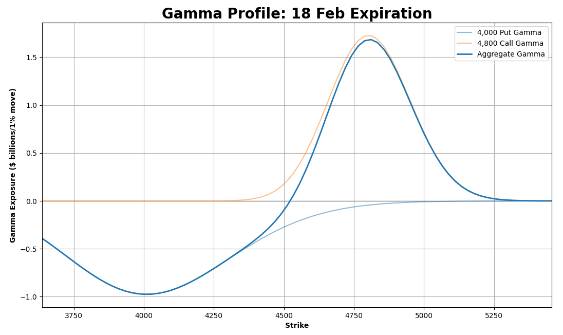
This gives us the following chart below. It shows the gamma exposure at each spot level resulting from this single option. As expected, it's lowest at the strike, and its gamma impact diminishes as we move closer to the current spot.
Ok, how about we add a few more in the mix?
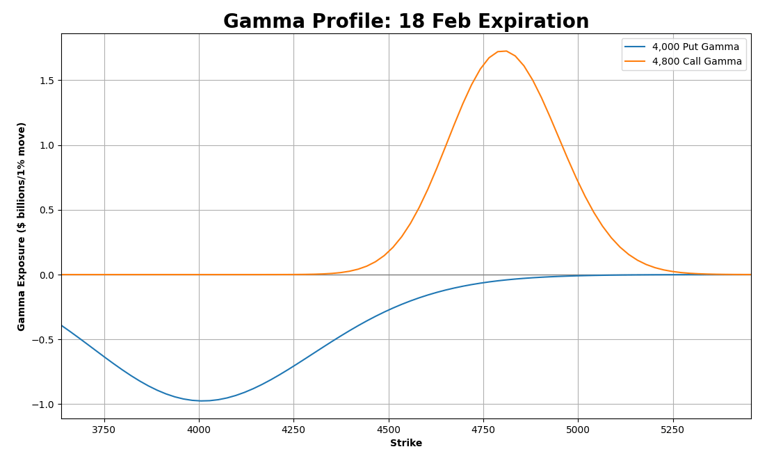
Enter 4,800 call...
Wow, she's absolutely gorgeous!
Sexy little thing... She gives you hope, but at the same time, keeps you at a distance.
She loves to tease...
Sorry, where was I?
Ah right. Now we have the gamma exposure for two options. As you can see, they have their own sphere of influence, sometimes offsetting each other. If we add them, we'll net out their impacts and get the overall gamma exposure.
Let's now throw in 4,300 put and 4,600 call.
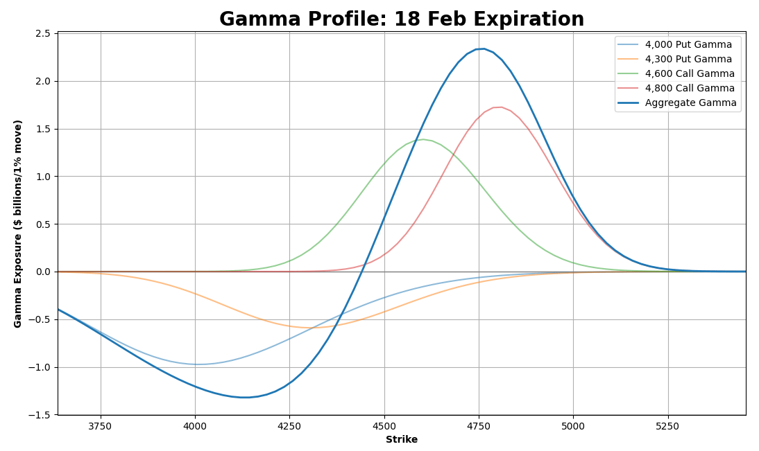
As we keep adding more options, we get a more complete picture of the gamma exposure for this expiration.
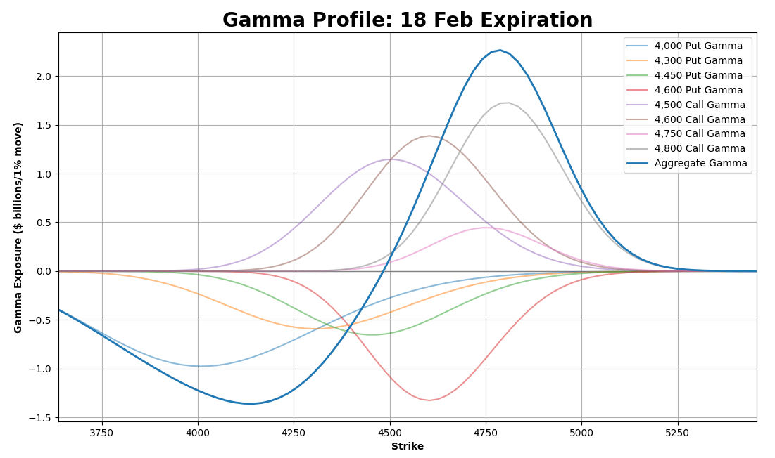
To get the overall gamma exposure profile, we'll need to do this exercise for all options across all expiries.
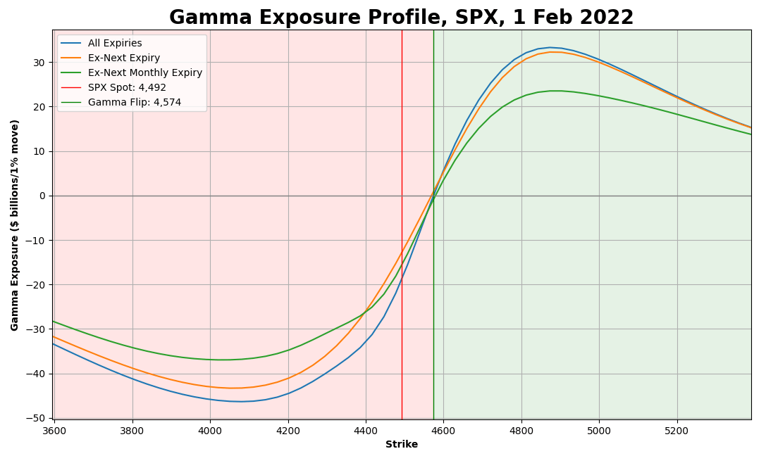
And if we do that, we'll get the following chart!
*drumroll*
Ta-da!
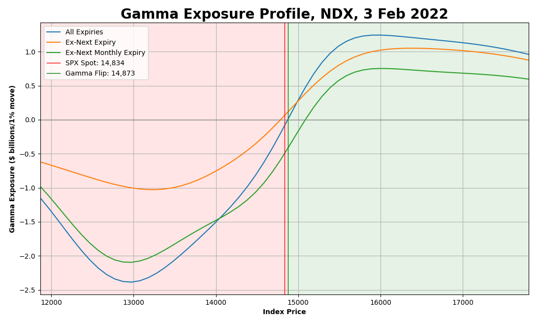
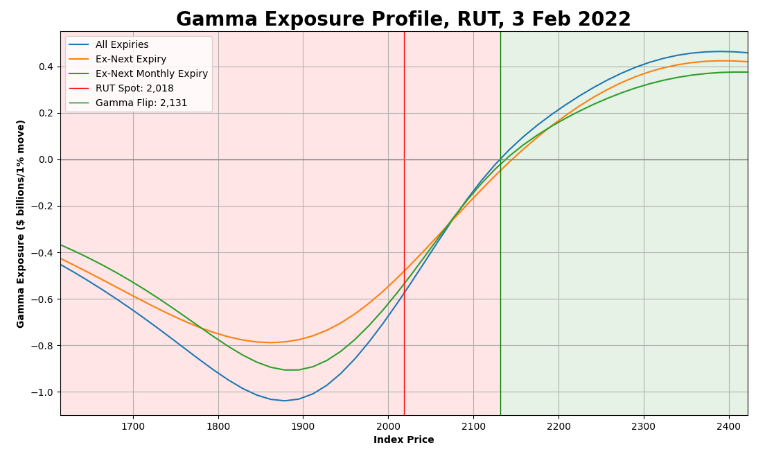
You might have seen this kind of chart before. It shows an approximate amount of dealer hedging flows across index levels, assuming the current state of the world.
Short gamma to the left.
Long gamma to the right.
Two levels are notable on this chart.
The first one is where the Total Gamma Exposure blue line crosses the current spot red line. This point represents the current spot gamma exposure and occurs at around -$19Bn. Yes, the same -$19Bn that we calculated earlier in Excel!
The second level is where the Total Gamma Exposure blue line crosses zero. On the chart, it occurs at around 4,575 SPX level. This is the Zero Gamma point, where the dealer gamma exposure flips from positive to negative.
Above this level, dealer hedging flows are stabilizing and add liquidity to the market.
Below this level, dealer hedging flows are destabilizing and add to the volatility instead.
At this level, flows are zero, as delta doesn't need rebalancing due to spot moves.
And now...
The moment we've all been waiting for!
The star of the show!
The one and only!
Please welcome!
The Python script that generates the gamma profile!
*applause*
import pandas as pd
import numpy as np
import scipy
from scipy.stats import norm
import matplotlib.pyplot as plt
from datetime import datetime, timedelta, date

pd.options.display.float_format = '{:,.4f}'.format

# Inputs and Parameters
filename = 'spx_quotedata.csv'

# Black-Scholes European-Options Gamma
def calcGammaEx(S, K, vol, T, r, q, optType, OI):
    if T == 0 or vol == 0:
        return 0

    dp = (np.log(S/K) + (r - q + 0.5*vol**2)*T) / (vol*np.sqrt(T))
    dm = dp - vol*np.sqrt(T)

    if optType == 'call':
        gamma = np.exp(-q*T) * norm.pdf(dp) / (S * vol * np.sqrt(T))
        return OI * 100 * S * S * 0.01 * gamma
    else: # Gamma is same for calls and puts. This is just to cross-check
        gamma = K * np.exp(-r*T) * norm.pdf(dm) / (S * S * vol * np.sqrt(T))
        return OI * 100 * S * S * 0.01 * gamma

def isThirdFriday(d):
    return d.weekday() == 4 and 15 <= d.day <= 21

# This assumes the CBOE file format hasn't been edited, i.e. table beginds at line 4
optionsFile = open(filename)
optionsFileData = optionsFile.readlines()
optionsFile.close()

# Get SPX Spot
spotLine = optionsFileData[1]
spotPrice = float(spotLine.split('Last:')[1].split(',')[0])
fromStrike = 0.8 * spotPrice
toStrike = 1.2 * spotPrice

# Get Today's Date
dateLine = optionsFileData[2]
todayDate = dateLine.split('Date: ')[1].split(',')
monthDay = todayDate[0].split(' ')

# Handling of US/EU date formats
if len(monthDay) == 2:
    year = int(todayDate[1])
    month = monthDay[0]
    day = int(monthDay[1])
else:
    year = int(monthDay[2])
    month = monthDay[1]
    day = int(monthDay[0])

todayDate = datetime.strptime(month,'%B')
todayDate = todayDate.replace(day=day, year=year)

# Get SPX Options Data
df = pd.read_csv(filename, sep=",", header=None, skiprows=4)
df.columns = ['ExpirationDate','Calls','CallLastSale','CallNet','CallBid','CallAsk','CallVol',
              'CallIV','CallDelta','CallGamma','CallOpenInt','StrikePrice','Puts','PutLastSale',
              'PutNet','PutBid','PutAsk','PutVol','PutIV','PutDelta','PutGamma','PutOpenInt']

df['ExpirationDate'] = pd.to_datetime(df['ExpirationDate'], format='%a %b %d %Y')
df['ExpirationDate'] = df['ExpirationDate'] + timedelta(hours=16)
df['StrikePrice'] = df['StrikePrice'].astype(float)
df['CallIV'] = df['CallIV'].astype(float)
df['PutIV'] = df['PutIV'].astype(float)
df['CallGamma'] = df['CallGamma'].astype(float)
df['PutGamma'] = df['PutGamma'].astype(float)
df['CallOpenInt'] = df['CallOpenInt'].astype(float)
df['PutOpenInt'] = df['PutOpenInt'].astype(float)


# ---=== CALCULATE SPOT GAMMA ===---
# Gamma Exposure = Unit Gamma * Open Interest * Contract Size * Spot Price
# To further convert into 'per 1% move' quantity, multiply by 1% of spotPrice
df['CallGEX'] = df['CallGamma'] * df['CallOpenInt'] * 100 * spotPrice * spotPrice * 0.01
df['PutGEX'] = df['PutGamma'] * df['PutOpenInt'] * 100 * spotPrice * spotPrice * 0.01 * -1

df['TotalGamma'] = (df.CallGEX + df.PutGEX) / 10**9
dfAgg = df.groupby(['StrikePrice']).sum(numeric_only=True)
strikes = dfAgg.index.values

# Chart 1: Absolute Gamma Exposure
plt.grid()
plt.bar(strikes, dfAgg['TotalGamma'].to_numpy(), width=6, linewidth=0.1, edgecolor='k', label="Gamma Exposure")
plt.xlim([fromStrike, toStrike])
chartTitle = "Total Gamma: $" + str("{:.2f}".format(df['TotalGamma'].sum())) + " Bn per 1% SPX Move"
plt.title(chartTitle, fontweight="bold", fontsize=20)
plt.xlabel('Strike', fontweight="bold")
plt.ylabel('Spot Gamma Exposure ($ billions/1% move)', fontweight="bold")
plt.axvline(x=spotPrice, color='r', lw=1, label="SPX Spot: " + str("{:,.0f}".format(spotPrice)))
plt.legend()
plt.show()

# Chart 2: Absolute Gamma Exposure by Calls and Puts
plt.grid()
plt.bar(strikes, dfAgg['CallGEX'].to_numpy() / 10**9, width=6, linewidth=0.1, edgecolor='k', label="Call Gamma")
plt.bar(strikes, dfAgg['PutGEX'].to_numpy() / 10**9, width=6, linewidth=0.1, edgecolor='k', label="Put Gamma")
plt.xlim([fromStrike, toStrike])
chartTitle = "Total Gamma: $" + str("{:.2f}".format(df['TotalGamma'].sum())) + " Bn per 1% SPX Move"
plt.title(chartTitle, fontweight="bold", fontsize=20)
plt.xlabel('Strike', fontweight="bold")
plt.ylabel('Spot Gamma Exposure ($ billions/1% move)', fontweight="bold")
plt.axvline(x=spotPrice, color='r', lw=1, label="SPX Spot:" + str("{:,.0f}".format(spotPrice)))
plt.legend()
plt.show()


# ---=== CALCULATE GAMMA PROFILE ===---
levels = np.linspace(fromStrike, toStrike, 60)

# For 0DTE options, I'm setting DTE = 1 day, otherwise they get excluded
df['daysTillExp'] = [1/262 if (np.busday_count(todayDate.date(), x.date())) == 0 \
                           else np.busday_count(todayDate.date(), x.date())/262 for x in df.ExpirationDate]

nextExpiry = df['ExpirationDate'].min()

df['IsThirdFriday'] = [isThirdFriday(x) for x in df.ExpirationDate]
thirdFridays = df.loc[df['IsThirdFriday'] == True]
nextMonthlyExp = thirdFridays['ExpirationDate'].min()

totalGamma = []
totalGammaExNext = []
totalGammaExFri = []

# For each spot level, calc gamma exposure at that point
for level in levels:
    df['callGammaEx'] = df.apply(lambda row : calcGammaEx(level, row['StrikePrice'], row['CallIV'],
                                                          row['daysTillExp'], 0, 0, "call", row['CallOpenInt']), axis = 1)

    df['putGammaEx'] = df.apply(lambda row : calcGammaEx(level, row['StrikePrice'], row['PutIV'],
                                                         row['daysTillExp'], 0, 0, "put", row['PutOpenInt']), axis = 1)

    totalGamma.append(df['callGammaEx'].sum() - df['putGammaEx'].sum())

    exNxt = df.loc[df['ExpirationDate'] != nextExpiry]
    totalGammaExNext.append(exNxt['callGammaEx'].sum() - exNxt['putGammaEx'].sum())

    exFri = df.loc[df['ExpirationDate'] != nextMonthlyExp]
    totalGammaExFri.append(exFri['callGammaEx'].sum() - exFri['putGammaEx'].sum())

totalGamma = np.array(totalGamma) / 10**9
totalGammaExNext = np.array(totalGammaExNext) / 10**9
totalGammaExFri = np.array(totalGammaExFri) / 10**9

# Find Gamma Flip Point
zeroCrossIdx = np.where(np.diff(np.sign(totalGamma)))[0]

negGamma = totalGamma[zeroCrossIdx]
posGamma = totalGamma[zeroCrossIdx+1]
negStrike = levels[zeroCrossIdx]
posStrike = levels[zeroCrossIdx+1]

zeroGamma = posStrike - ((posStrike - negStrike) * posGamma/(posGamma-negGamma))
zeroGamma = zeroGamma[0]

# Chart 3: Gamma Exposure Profile
fig, ax = plt.subplots()
plt.grid()
plt.plot(levels, totalGamma, label="All Expiries")
plt.plot(levels, totalGammaExNext, label="Ex-Next Expiry")
plt.plot(levels, totalGammaExFri, label="Ex-Next Monthly Expiry")
chartTitle = "Gamma Exposure Profile, SPX, " + todayDate.strftime('%d %b %Y')
plt.title(chartTitle, fontweight="bold", fontsize=20)
plt.xlabel('Index Price', fontweight="bold")
plt.ylabel('Gamma Exposure ($ billions/1% move)', fontweight="bold")
plt.axvline(x=spotPrice, color='r', lw=1, label="SPX Spot: " + str("{:,.0f}".format(spotPrice)))
plt.axvline(x=zeroGamma, color='g', lw=1, label="Gamma Flip: " + str("{:,.0f}".format(zeroGamma)))
plt.axhline(y=0, color='grey', lw=1)
plt.xlim([fromStrike, toStrike])
trans = ax.get_xaxis_transform()
plt.fill_between([fromStrike, zeroGamma], min(totalGamma), max(totalGamma), facecolor='red', alpha=0.1, transform=trans)
plt.fill_between([zeroGamma, toStrike], min(totalGamma), max(totalGamma), facecolor='green', alpha=0.1, transform=trans)
plt.legend()
plt.show()
All you need to do is download the "quotedata.csv" file from CBOE for whatever index you want.
Put it in the same directory as the script.
Run it.
And sit back and relax.
Let the script do it all for you.
Easy.
For example, do you want some gamma for $NDX?
Voila!
Russel 2000?
Bam!
You can also adapt the script and feed your data into it, or change any of the inputs or assumptions.
UPDATE 1: If the code doesn't work: Depending on your region and time/date settings, the CSV file might be formatted differently. If that's the case, the code won't be able to parse it correctly and will give an error.
If you run the code and it doesn't work, please try it with this file:
UPDATE 2: You can bypass various CSV file formatting issues by downloading data directly into Python from CBOE API, without going via the CVS file.
This can be done using the updated code below:
The script also takes in command line arguments. To run the script, you need to specify the index ticker that you want to calculate the gamma for. For example, the following command will run the script for SPX:
$ python gammaProfileCommandLine.py SPXThanks for reading, and I hope it was helpful!
Feel free to follow me (@perfiliev) for more educational threads around stocks, options and other topics within financial markets.
In case you enjoy watching videos, I'd like to invite you to my YouTube channel, where I also cover various financial topics.
Thank you for reading!


